
The Challenge
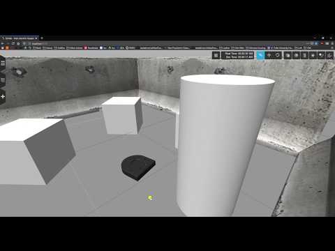
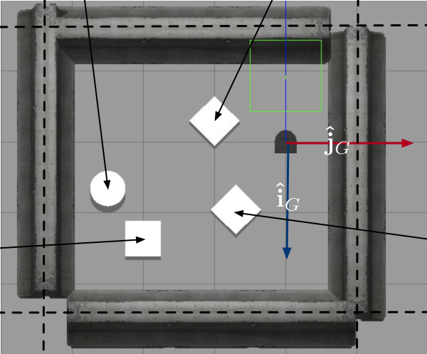
The Gauntlet challenge is to navigate a robot successfully from a starting position in to the “Bucket of Benevolence” (The cylinder) in a simulator. The challenge is to avoid the walls and obstacles present in the Gauntlet. See the picture below for what the Gauntlet looks like:
High Level Plan (See code and implentation section for more details)
- Use the robot’s Lidar to obtain data about surrounding area
- Parse Lidar to detect features
- Use RANSAC algorithm to find circles and lines/walls
- Build a potential field with sources around lines and sinks around the BOB(Bucket of Benevolence)
- Calculate Gradient of potential field at robot location and drive accordingly using gradient descent
Results
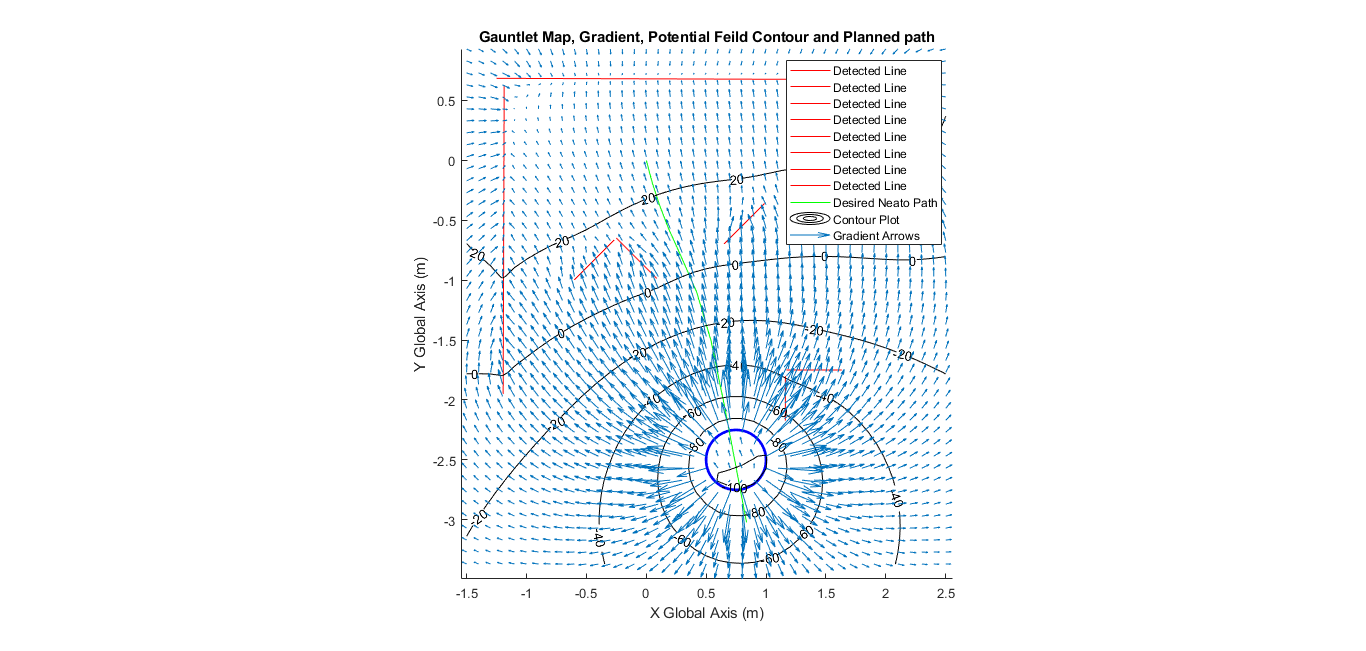
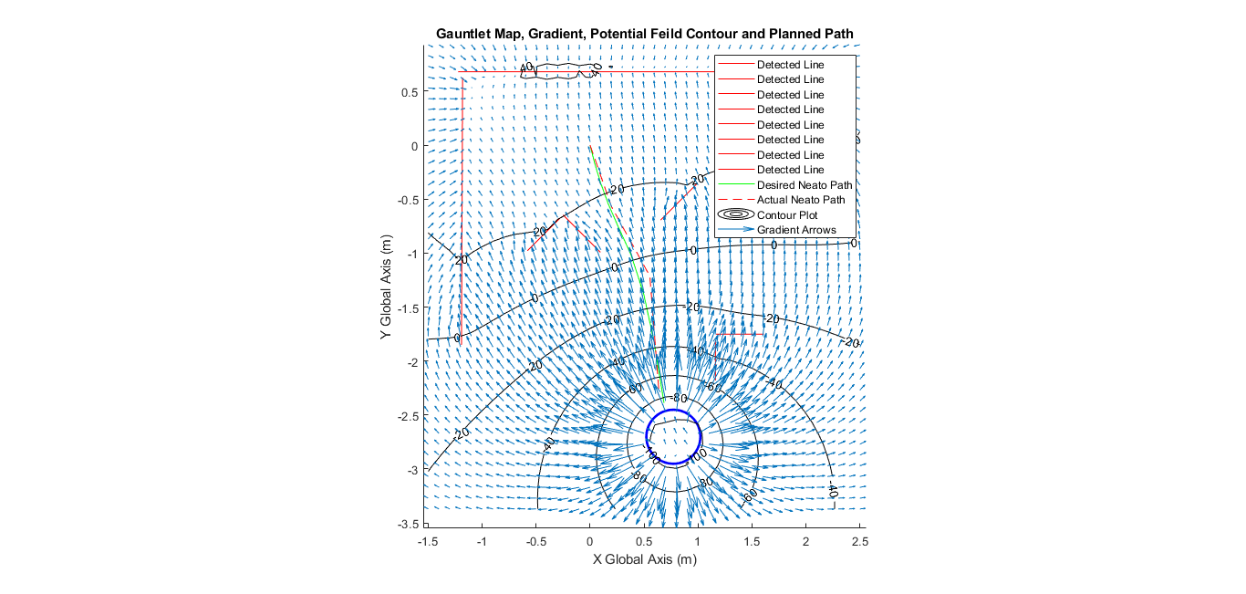
This final plot was generated with encoder data recorded from the robot. It also appears that the robot took ~25 seconds to get to the BOB. This was a long time, the driving time is certainly less. This is due to the fact that it is scanning between each drive step and re-calculating the topography etc. This also explains why my actual plot is slightly different than the calculated plot that was made off of a single scan at the starting point. If navigating with a set path rather than re-scanning than implementing a parametric curve fit to the set points would have allowed for an implemantation of drive control that could go faster rather than driving small segments of straight lines
Implementation Strategy and Code
IN PROGRESS For the code: View Code Please excuse this code, it is made to be able to retrieve scans in the globabl frame to plot things nicely, and parameters must be changed to drive in time steps with relative LIDAR scanning. Plotting the final path must be uncommented and ran with global frame settings with driving disabled
Broken down from into the main points above:
Use the robot’s lidar scanner and parse scan to detect features
The scan data returned from the robot contains 360 datapoints, each recording a distance to an object at each degree of rotation of the scanner. For points in which nothing was seen zero is returned. This data is then cleaned to remove zeros. The data is also offset to the lidar scanner, this data gets converted to cartesian coordinates and translated so that the origin is centered on the robot’s wheelbase.
How to detect walls/lines in scan data
There are several options here. We explored using simple linear regression on all points and PCA(Primary Component Analysis). These can yield decent results if the data only contains one feature. This leads to why RANSAC is so powerful. See explanation below,
How RANSAC Works
RANSAC stands for Random Sample Consensus. This is a method in which to determine a best fit of data by minimizing outliers. The easiest way to show how this works is to walk through an example for looking for a line in a set of data points. The first step is to randomly sample 2 points (the minimum needed to define a line). Calculate an equation for the line between these two points. Get sum of the number of points within a threshold distance of the line (measured normal to the line). THese are called inliers. If the number of inliers is higher than a previous number of inliers then set this set line as the most difinitive line in the dataset. Repeat this for a number of iterations (to ensure you sample enough random points to capture lines within the data). Take the final line and store data about is and then remove all points that are inliers for that line from the main dataset. This essentially will allow you to repeat ransac multiple times until you run out of points in the scan(have determined all the lines.) Please note this descibes the most basic application of a ransac algorithm. In pseudocode:
Clean Scan

while there are points in the scan
  set max inliers to zero
  initalize best line
  for a number of random samples
      grab two random points from a scan

      determine the line between them

      calculate number of points in scan data that are within threshold (inliers)

      if number of inliers is greater than the max inliers
        these points define the new best line!!
        set outer max inliers value to num of inliers
        set best line to these line parameters

  Remove best line inliers from main scan data
  Add line data to colleciton of detected lines
Applications to Circles/Arcs and Lines
Above shows how RANSAC can be used for detecting lines. All that changes in RANSAC for other types of functions are the number of points sampled and the method for determine inliers. In our case we calculate what circle best fits 3 points and then examine how many points are within threshold distance to the circle.
Problems with RANSAC and how they were addressed
One problem that occured was that lines that intersected at 90* angles looked like circles to this algorithm.A collection of some side points that were straight were in the threshold to look like a valid circle. This seemed like a nasty problem, and it was solved by doing ransac on the points that were inliers of the “found” circle. If these points on the circle actually were a circle than the calculated radius and center wpuldn’t change position much. However, in the case of having two lines looking like a cirlce one iteration of ransac would look hugely different from the “found” result. If there was a large discrepancy then I assumed this was misidentified. Similar accuracy might be acheivable by simply tightening the threshold of the circle.
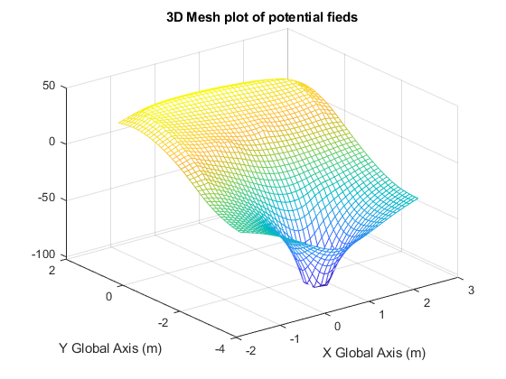
Build a potential field with sources around lines and sinks around the BOB(Bucket of Benevolence)
The plan to navigate this obstacle course is to use gradient descent. For this to be possible there must be a function defined across the x,y grid of our map with a “height” and where the steepest direction down the topography indicates the way to the BOB and away from obstacles. This is accomplished using one simple fucntion to build a point source(high point) or sink (low point): f(x,y) = ln(sqrt((x-a)^2+(y-b)^2)). This creates a sink around the coordinates (a,b) to create a source this cuntionally is negated. To create line sources multiple point sources can be combined together in one function. ie: f(x,y) = ln(sqrt((x-a)^2+(y-b)^2)) - ln(sqrt((x-c)^2+(y-d)^2)). To build source and sinks these fucntioned are chained around a circle with a small spacing between points or with multiple points along a line.
Problems with my potential field generation
This is definitely a valid way of generating potential fields. However, it doens’t do the best job at making the line segments. The nature of these potenital fields is to act as points and add or subtract from everythign else around them. This transaltes to a peak in the middle of a line segment. This doesn’t seem to be desired behavior. It is more important to avoid the edges ob objects than the middles. Line’s cna liekly be built in a more logical way that makes them more equal
Calculate Gradient at robot location and drive accordingly using gradient descent A massive function is created that represents the “topography” of the gauntlet. Obstacles are high points and the BOB(destination) is the low point. Driving directions are calculated based on the negative gradient vector, which points towards the steepest descent, which in should correlate to a path that heads towards the destination and avoids obstacles. This vecor is scaled to an appropriate drive distance and then the robot changes it’s orientation and drives the distance. This is done by driving the robot based on time (angular velocity and total angle change can be calculated). Distance is also driven based on time since wheel speed is known. I also tested using the simulator’s encoders with little to no increase in results. Stopping the robot is achieved by listening for a bump on any part of the robot!
How I would do this differently
- Implement a “search” drive sequence purely to build a map of the room to navigate with
- Calculate potential fileds in a more robust way (so that the top of a wall was “flat” and less computation time, not symbolicly maybe)
- Interpret evrything in the global frame
- Record position of oreintation of robot during navigation (required to interpret in global frame)
- Add scans and data together (store and filter lidar data to build a better map of gauntlet as you travers)
- Move robot between multiple small points according to gradient, along a curve that was fit to the points
- This would allow for more accurate encoder path reconstruction.