
Abstract/Introduction
This project aims to implement a shortest path finder at a small scale: using the Olin college campus. In OlinMaps, we sought to explore path planning between multiple points in the way that sites such as Google Maps are able to do, and show how it is done.
Once a map reaches a certain size, it is not viable to test all possible routes from a start point to an end point, so we utilize algorithms to reduce the search space. The field of path planning is well studied, with several algorithms - namely Dijkstra’s and A* - that are directly applicable and well documented that we can apply towards our problem.
To use the finished product in a Jupyter Notebook, click here.
Project Design
This project is comprised of three main parts:
- A graphical representation of Olin
- An A* implementation that uses our graph to determine the optimal route between two or more locations
- A visualization of the A* algorithm and the calculated shortest path
Graph Creation
In order to create the graph, we traveled to different areas of Olin’s campus that might be of interest to Oliners, dropped a pin at each location using Google Maps, and compiled a list of nodes from the longitude and latitude coordinates of the pins. These points make up the destination nodes of the graph that the user might choose to travel between, such as the different entrances and exits of East Hall or the Academic Center. We also used intermediary pathway nodes (such as sidewalk intersections) to connect the destination nodes, mapping our graph closely to the physical layout of Olin’s campus.
Using the Google Maps pins and their longitude and latitude data, we calculated the distance between the nodes by using a haversine function. These distances served as edge weights in our graph. This distance calculation assumes a flat map and does not account for elevation changes. Thus, our implementation considers Olin’s campus in only two dimensions, but since the campus is fairly flat it is a decent estimation of distance for the majority of paths.
We used the Networkx Python package, a ready-to-use graph generation framework, to create and manipulate this graph.
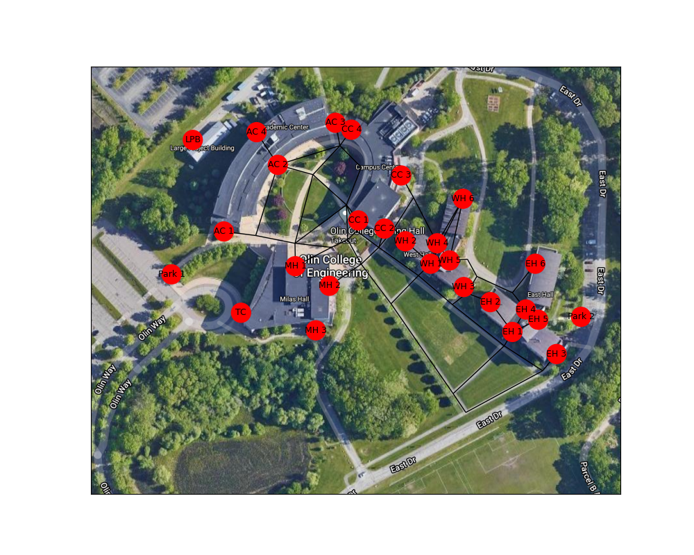
Figure 1: A visual representation of the entire graph overlayed on an image of Olin’s campus
A* Algorithm
Our implementation is loosely inspired by Google Maps’ use of Dijkstra’s algorithm as its path planning solution, which is detailed in this article. The algorithm used in our implementation, A*, is an adaptation of Dijkstra’s algorithm that uses a heuristic to improve efficiency by selectively exploring possible paths according to the distance each path improves toward the destination. The heuristic we used for the A* algorithm is the Euclidean distance between the current node and the destination node, which is calculated using each node’s longitude and latitude coordinate pair in. This heuristic acts as a metric for the optimality of a potential path. We used parts of the code from Homework 9 in our implementation of A*.
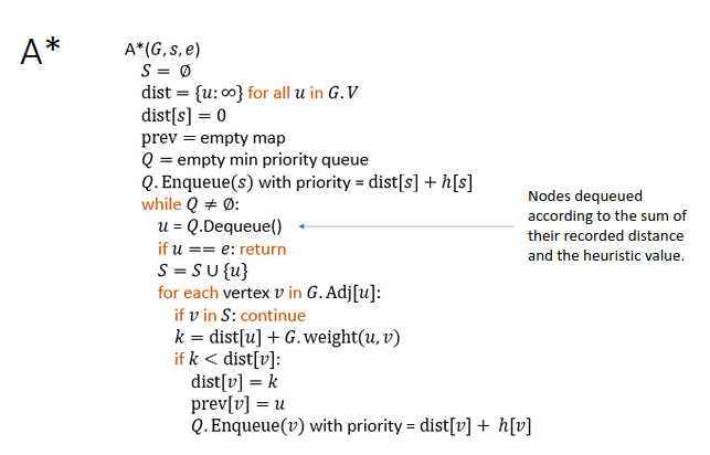
Figure 2: A* pseudocode
The above pseudocode (credit to DSA Teaching team) was used to create our implementation of A*. The algorithm has two main sections: the setup section and the searching section. In the setup section, we initialize various variables used by the searching section of this algorithm. These include sets to contain the shortest distance to each node and nodes that have already been visited. We also initialize a PriorityQueue that is used to prioritize nodes that will get us closer to our destination while exploring the graph.
In the searching section, the graph is explored until a solution is found or there are no nodes left to explore. The algorithm works by dequeuing a node from the priority queue on each iteration. A node’s priority is determined by the estimated distance to the destination node (via current travelled distance and the heuristic). Adjacent nodes that have not been visited are explored as well. If this route to the nodes is the shortest path, these nodes are added to the queue with a priority based on the distance to the node and the heuristic to the final destination. There is also a dictionary mapping previous nodes for a given node. This allows us to reconstuct the path taken once the destination is reached. This loop continues until the destination is located or the graph is fully explored. For a more in-depth explanation of A*, see this GeeksforGeeks article.
Visualize the Algorithm
Creating a visualization and simple interface for our path planning program was important to ensure that OlinMaps would be usable to Oliners. To do this, we superimposed the Networkx graph of the calculated shortest path on a satellite image of Olin’s campus (the intermediary pathway nodes are not typically of interest to the user, so are not labeled in the visualization). This allows users to easily view the optimal path and offers a visual representation of how the A* algorithm determined it. The visualization also helped us debug our A* algorithm and validate our results visually.
The animated aspect of the visualization uses the user’s start and end location selection as input for the A* function along with the Networkx graph containing the named coordinate pairs. The A* function returns a list of nodes that comprise the shortest path solution and a list of sets that contain the nodes explored during each step of the route-optimization process. The nodes in each set are then plotted on the satellite image of Olin using Matplotlib and Networkx’s draw function and saved. Afterward, the shortest path is plotted and saved. The figures are then stitched together sequentially into a GIF using the ImageIO Python module.
Figure 3: Example route finding animation from East Hall to the AC
Analysis
If you would like to test the code out yourself, click here.
Below is an animation generated using our path planning program. It shows the best path from the door of the AC nearest the traffic circle to the main entrance to East Hall.

Figure 4: Shortest path between the West door of the AC to the main entrance to East Hall
In the figures below you can see more examples of our algorithm planning routes between points. Based on our own experiences walking around campus, the routes chosen tend to be the most efficient way to get between the two points.
Figure 5: Shortest path from the West entrance to the Academic Center to the lower level of the Campus Center
Figure 6: Shortest path from the Lowest exit of East Hall to one of the Campus Center entrances
The A* Heuristic
Our implementation employed A*, a heuristic algorithm, to determine the optimal path between two points. For a heuristic, we used the Haversine Python package to compute the Euclidean distance between the longitude and latitude coordinate pairs of the current node and the destination node. The Euclidean distance between two points is the shortest distance “as the crow flies,” meaning that even if the current node is adjacent to the destination node, the heuristic distance is equal to the actual distance travelled from the current node to the destination node.
In cases where the current node is not adjacent to the destination node, the heuristic distance is less than the actual distance that will be travelled to get from the current node to the destination node, since the destination node must be accessed via at least one intermediary node. The only exception is the case where the intermediary node falls along the Euclidean path between the current node and the destination node, in which case the heuristic distance is equal to the actual travelled distance. In any scenario, the heuristic distance is less than or equal to the actual distance, making it admissible.
Limitations of Our Algorithm
One limitation of our implementation is that the A* algorithm is not guaranteed to produce the most optimal solution as it does not consider every possible sub-problem. As a heuristic algorithm, it is more likely to return an *approximately* optimal solution, while greedy algorithms are more likely to return optimal solutions. An alternative greedy path planning algorithm we could have used is Dijkstra’s algorithm, which operates similarly to A* but does not use a heuristic to focus its exploration, considering all subpaths at each node, even if they are unlikely to result in an optimal solution.
Another limitation of our algorithm occurs when it is presented with a multi-stop route optimization problem. Finding the optimal path and order in which to visit multiple destinations is essentially just the age-old Travelling Salesman Problem, which is NP hard according to GeeksforGeeks. However, if the optimal order to visit the destinations is given, our algorithm can successfully find an optimal path. This is because the optimal path of an ordered trip is equal to the sum of the optimal paths between the listed nodes.
Future Goals/Direction of work
One way we could improve the accuracy of our optimal route finder is by defining obstacles rather than paths around them. This might also make map data storage more efficient and create more appealing visualizations with less choppy looking paths.
Another way we could improve our program is by using some form of stop ordering logic to calculate more optimal routes for multi-stop trips. Currently, the program handles multi-stop trips by running the A* algorithm on every pair of stops (meaning the first stop is used as the start node and the second as the end node, then the second stop used as the start node and the third as the end node, and so on) in the order they are entered. For smaller multi-stop problems, we might instead choose to find the route lengths of all possible stop orderings using the current method and determine the best route. For larger multi-stop problems, we could sort the stops into groups by location and then compute a fairly optimal route by using the solution described for smaller multi-stop problems on each group.
We might further optimize our route finder computationally using caching. We could store the distances between frequently used nodes to avoid calculating the same distances repeatedly. We could also account for cases where one sub-path is consistently faster than others. For example, if the shortest path to AC 4 (see Figure 1 for location key) is always through AC 2 except when starting from the LPB, we could include a condition that automatically chooses to access AC 4 via AC 2 unless the start node is the LPB, avoiding any excess distance calculations.
One way that we could expand upon this project is by incorporating elevation into our shortest path calculation. Using elevation in addition to horizontal distance to determine the most optimal path was one of our stretch goals, and might make our program more accurate when determining the shortest path between locations. This would also allow us to determine the shortest path between rooms on different floors in buildings, which would be useful when travelling between classes. Information like this could also be used to improve evacuation routes, resulting in a safer environment.